Relativistic Radiation Magnetohydrodynamics
The radiation field is one of the most important ingredient in high-energy astrophysical phenomena. For example, the radiation pressure strongly affects on the accretion disk dynamics and it supports the gravity by the central black-hole in supercritical or sub-ciritical (super-Eddington) accretion flow. Also, radiation field is important in the point of view of explaining observational results from numerical simulations. In this page, we briefly summarize the difference between models that approximately treat the radiation field.
Time evolution of radiation field is described by radiation transfer equation, which is the Boltzmann equation for the photon field.
where \( I_\nu, S_\nu\) are the intensity and source function and \(n^j\) is the unit vector. Solving the radiation transfer equation coupling with hydrodynamic equations is the challenging task for the comunittee of high-energy astrophysicist. The intensity has a 7 independent variables, i.e., time, position, and photon momentum. For expanmple, if we'd like to solve a transfer equation with 100 grids in each space, we need memory more than 100GB. Such a huge memory cannot be available in current supercomputers. Thus we want to reduce independent variables. By integrating equation (1) in the momentum space, we obtain zero-th order moment equation,
\[ \frac{\partial E_r}{\partial t} + \frac{\partial F_r^j}{\partial x^j} = \rho \gamma(j' - c \kappa' E'_r) - \rho \gamma (\kappa' + \sigma')\frac{v_j F_r'^j}{c}, \]where \( E_r, F^j_r\) are the radiation energy density and flux. \( \kappa \) and \( \sigma\) are the absorption and scattering coefficients. Here a dash denotes for the quantity defined in the comoving frame. When multiplying equation (1) by \( n^i\) and integrating it in momentum space, we obtain 1st order moment equation,
\[ \frac{1}{c^2} \frac{\partial F_r^i}{\partial t} +\frac{\partial P_r^{ij}}{\partial x^j} = -\rho \gamma \frac{v^i}{c^2}(j' - c \kappa' E_r') - \rho \gamma (\kappa' + \sigma') \frac{\gamma v^i v_j F_r'^j}{(\gamma+1)c} - \frac{1}{c} \rho (\kappa' + \sigma') F_r'^i, \tag{2} \]
where \( P_r^{ij} \) is the radiation pressure tensor. Not that since we integrate the intensity in the momentum space, only 4 independent variables (time and position) remains. Thus the required memory size and computational costs are comparable to those of fluids. We can solve radiation moment equations coupling with fluids consistently.
As the same as the fluid approximation, equations (1-2) are not closed but we need to specify an explicit form of \( P_r^{ij} \), which corresponds to the equation of state for the radiation field. In the following, we show two examples of a simple form of \( P_r^{ij} \).
Diffusion (Eddington) Approximation
In the Eddington approximation, radiation field is assumed to be isotropic in the comoving frame. This leads to
\[ P'^{ij} = \frac{\delta^{ij}}{3} E'_r.\]where \(P^{ij} \) is the radiation stress and \(E_r\) is the radiation energy density. These quantities should be evaluated in the comoving frame.
M-1 closure
In the formulation of M-1 closure, it is allowed that the radiation field can be anisotropic in the comoving frame. Then the radiation stress is given by
\[ P^{ij}= \frac{1-\chi}{2}\delta^{ij} + \frac{3\chi-1}{2}n^i n^j \]where\(n^i\) is the unit vector parallel to the radiation flux (Levermore '84). \(\chi\) and \(\n^i\) are functions of \(E_r\) and \(n^j\).
Caldera problem in 2D
Now, I'd like show difference between the Eddington and M-1 closures.
At the initial state, radiation energy is confined within \( r < 0.1 \). As time goes on, (\ E_r\) expands in a optically thin medium, forming a caldera structure. In this test, the Eddington approximation is applied.
In the similar method of Flux Limited-Diffusion approximation (FLD), such a caldera structure cannot be recovered since the radiation flux is assumed to be proportional to the gradient of \( E_r \). In this case, the radiation energy evolves according to the diffusion equation. The FLD approximation is valid in a optically thick medium, but is not suit to the wave propagation in an optically thin medium. In the Eddington approximation, which is also valid in an optically thick case, the caldera structure is recovered since we solve the time evolution of \( F_r\). Then, equation (1-2) becomes wave equation (or telegraphic equation with a finite opacity). With this view, Eddington approximation is more reasonable tan the FLD approximation.
We note that the wave velocity in the Eddington approximation reduces to \( c/\sqrt{3} \) since the isotropic radiation pressure is assumed. This is the same with the sound velocity of relativistic gas. Thus, The Eddington approximation is not enough to describle the wave propagatin in an optically thin medium.
For the M-1 closure, the wave velocity successfully approaches to the light speed in an optically thin medium (not shown, but we can understand from equations [1-2] by taking \( \kappa' = \sigma' = 0 \). Thus the M-1 closure is the best approximation to describe radiation field in the limit of optically thick and thin cases.
pulse collision in 1D
The radiation flux Fr is given by |Fr| = c Er for the M-1 model and |Fr| = c Er/3 for the diffusion model. When the radiation fields collides each other, the radiation passes in the Eddington model. In the M-1 model, however, wave profiles are more diffusive after they passes each other. This is because the Eddington tensor becomes isotropic when \( F_r=0\).
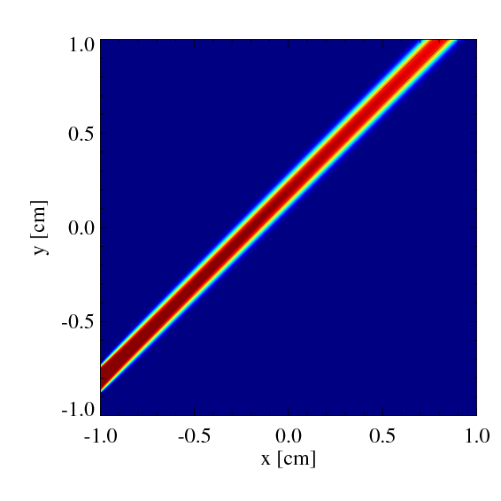
beam
Radiation is injected at x=-1 and y=[-0.875,-0.750], while the radiation flux is given by (\(F_x, F_y, F_z\)) = (\(cE_r/\sqrt{2}, cE_r/\sqrt{2}, 0\)). Optical depth of the system is much smaller than unity. Color shows the radiation energy density. We can see that the light propagates in straight. The radiation passes the boundary with a small reflection.
go back to page top
two beams
Radiation is injected at x=-1, +1 and y=[-0.875,-0.750], while the radiation flux is given by \( (F_x, F_y, F_z) = (cE_r/\sqrt{2}, \pm cE_r/\sqrt{2}, 0) \). Optical depth of the system is much smaller than unity. Color shows the radiation energy density. We can see that the light propagates in straight. We note that the radiation does not pass each other when they collides. This is because the flux \(F_x\) becomes zero, leading to that the trace of the Eddington tensor becomes below unity. In the formulation of M-1 closure, the radiation stress tensor \(P^{ij}\) is determined only \(E_r \) and \(F\), but it is independent of the optical depth. This means that the closure relation approaches that of the diffusion (Eddington) approximation when the flux vanishes even when the system is optically thin. This is the main problem for the M-1 closure. To overcome this problem, we might take into account the optical depth on the closure relation.
In this simulation, the ratio of the radiation energy injected from right and left boundary is 7/3. We note that the radiation does not pass without interaction but the radiation energy becomes diffusive. In the symmetric case, \(F_x\) becomes zero at which two radiation trajectories across. In the asymmetric case, \(F_x\) does not become zero but it has a negative value. However, the radiation becomes diffusive since the trace of the Eddington tensor becomes less than unity as well as the symmetric case.
shadow problem
Radiation is injected from the boundaries x =-0.5cm in a optically thin media (optical depth of 0.15. There is a clump at the origin whose optical depth is 10000 times larger than that of the background optically thin media.
The color shows the radiation energy density. The Eddington approximation (diffusion limit) is adopted in the model of upper panel, while the M-1 closure is implemented in the models of middle and bottom ones. The approximate Riemann solver is used in the bottom panel which takes into account the the propagation of the wave front.
In the diffusion limit, the wave front propagates with the speed c/√3, while it has a light speed c in the M-1 closure.
Due to the diffusion approximation, the radiation field comes around behind the clumps and there are no shadow. On the other hand, the shadow can be recovered with the M-1 closure relation.
Since equations are solved in the 2nd order accuracy in space, we cannot see the difference between the middle and bottom one. But the bottom one is more accurate about 10% than the middle one. This is because the middle one is solved by Lax-Friedreich method (i.e., constant characteristic wave velocity in HLL method), while the wave velocity is calculated in the bottom one).
shadow problem in the cylindrical coordinates
The radiation is injected at \( r=1 \) cm with a constant luminosity. There are four clumps whose optical depth is about 10, while the optical depth in the ambient plasma is 0.01. The figure in the domain of \(\theta=[-\pi/2,\pi/2]\) shows the result with the M-1 closure, while that of \(\theta=[\pi/2,3\pi/2]\) shows the results with the Eddington approximation.
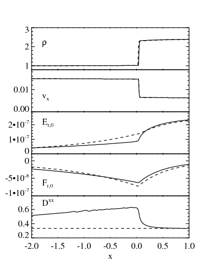
non-relativistic strong shock
go back to page top
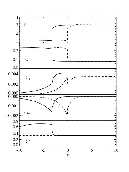
mildly relativistic strong shock
go back to page top
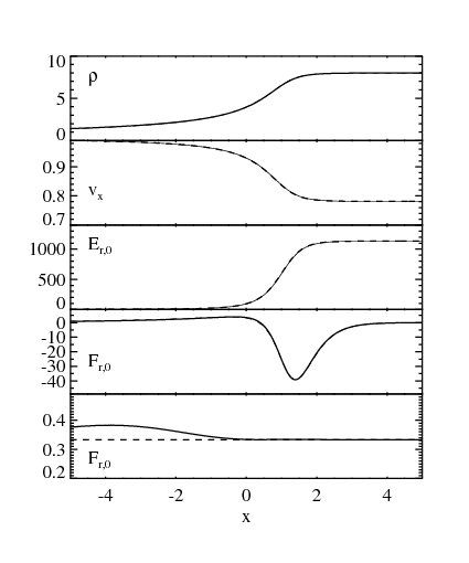
highly relativistic strong shock
go back to page top
radiation dominated shock

go back to page top